
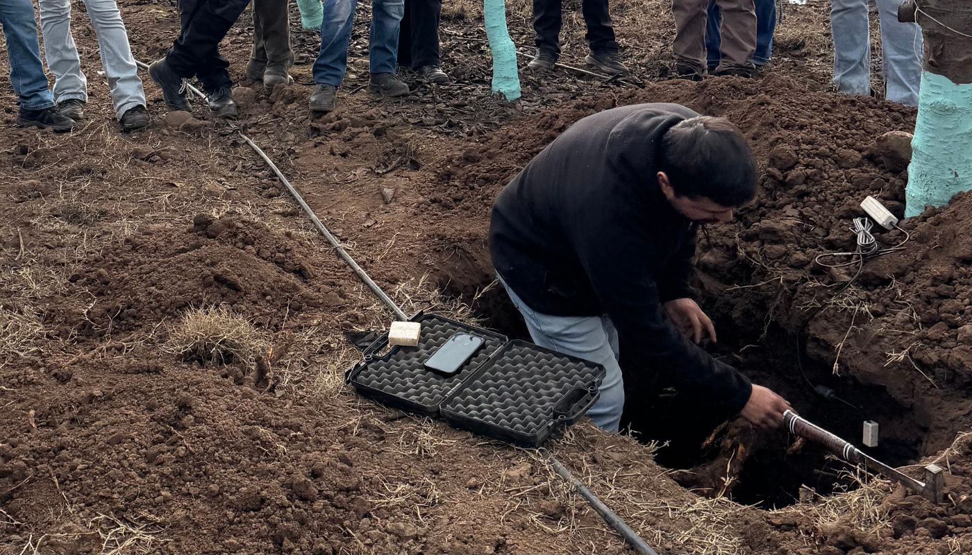
The three questions at the start of the season remain the same: when to begin irrigating, how much water to apply per irrigation event, and the frequency of irrigation. What has changed in recent years is not the questions themselves, but the amount of information available to answer them: properly executed soil pits, flow measurements, probes, and proprietary weather stations allow us to replace guesswork based on habit with hard data.
1. The Legacy of Winter: Soil Retention Capacity Dominates
The timing of the first irrigation is not determined by the calendar, but by the moisture present in the soil profile. Soil retention capacity and the date of the last rainfall event define how much water remains available and for how long. In soils with high retention capacity, late rainfall can delay the first irrigation by several weeks; in light soils, that same moisture is depleted within a few days.
The difference is significant, and it is best to measure it rather than estimate it. Based on the texture of each soil horizon, one can estimate field capacity and the permanent wilting point; these figures allow for the calculation of available water and the specific moisture level at which irrigation should resume.
Table 1. Available water and irrigation threshold by soil texture. Adapted from Saxton and Rawls (2006).
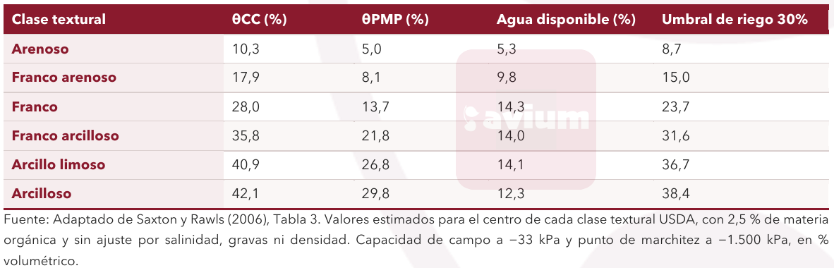
The values in the table above are for reference only and may vary depending on the sensor type (FDR, TDR, ADR, etc.). It is important to establish specific reference values for each individual case, as sensors estimate volumetric soil water content using “calibration” equations applied to raw data derived from the soil’s dielectric permittivity. Comparing this value against in-situ soil pit observations and their dynamics is key to interpreting the data and making objective decisions.
The final column shows the volumetric soil water content based on a 30% irrigation threshold. This represents the moisture level at which irrigation should begin if 30% of the available water is allowed to be depleted; it is the figure primarily compared against the sensor reading. Generally, irrigation criteria for cherry trees are based on a depletion of 30% to 40% of available soil moisture.
Another factor determining when to start irrigation is infiltration. Low-lying areas—characterized by a high water table and/or compacted soil layers—accumulate water that fails to drain. In these spots, excess water leads to oxygen deprivation, root death, increased disease pressure, and ultimately, phenological unevenness within the same orchard block. Satellite imagery and other tools that characterize spatial variability help delineate these zones before the season begins, allowing for continuous monitoring and site-specific management—provided the variability is significant enough that taking action would benefit production potential and fruit quality.
2. When should irrigation begin? Three signals that must coincide
The first irrigation is warranted when three signals coincide: soil moisture is below field capacity and approaching the irrigation threshold; the soil has reached a temperature that allows root growth to begin; and the plant has developed sufficient leaf area to actively transpire.
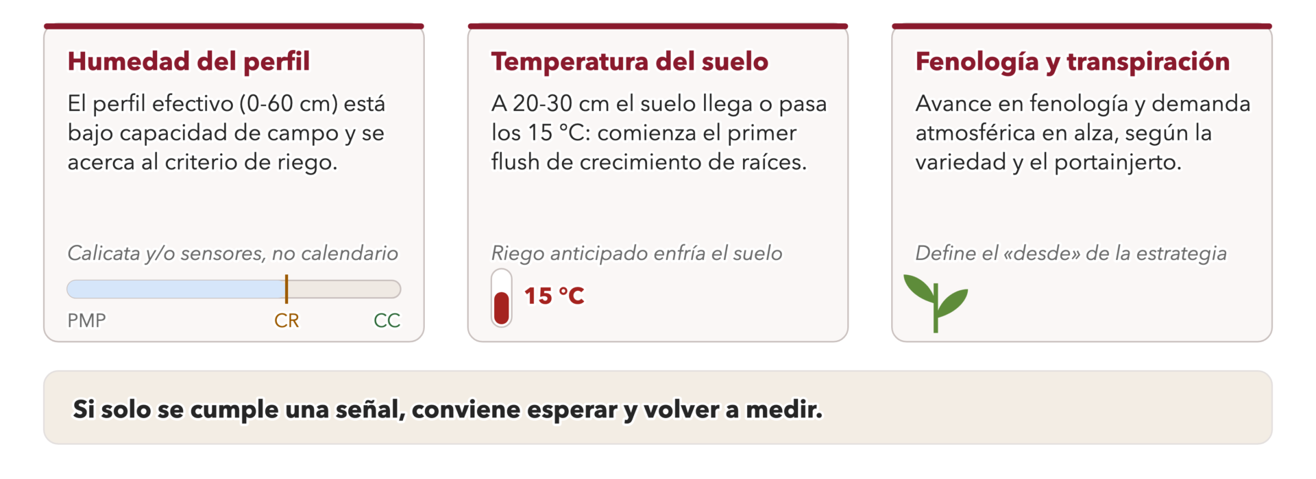
Soil temperature
The first flush of root growth begins when soil temperatures reach or exceed 15°C within the top 20–30 cm of the soil profile. Early irrigation lowers the profile temperature due to water’s high specific heat capacity.
3. How much to irrigate? The soil reservoir, not the clock
The amount of water applied during each irrigation event is determined by volume (mm) rather than duration (time). First, the soil profile’s water-holding capacity within the effective root zone is calculated; this volume is then converted into irrigation time based on the system’s application rate. In practice, however, the reverse approach—observing the depth a given irrigation run reaches over time—can also yield the same practical conclusions.
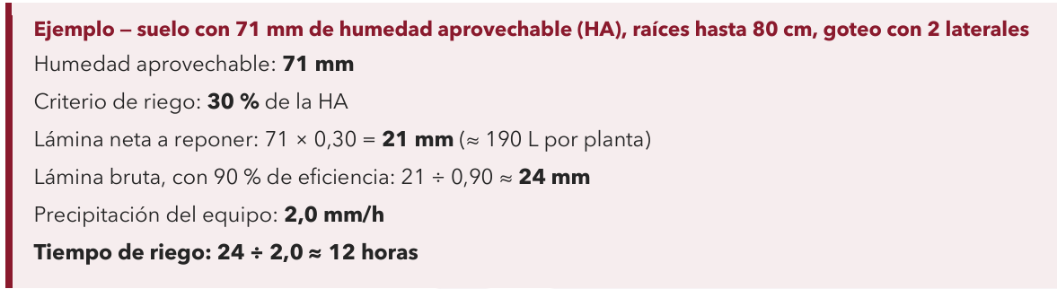
The same example illustrates the depth reached by each irrigation event. Starting from the soil surface, the water moves downward at a rate of approximately 7 cm/hour; thus, after 8 hours, it reaches a depth of about 54 cm; after 12 hours, it reaches 80 cm—covering the effective root depth in this example—and after 14 hours, it descends to a depth of approximately 1 m (these estimates assume a completely homogeneous soil texture, with no compacted layers or significant stone content).
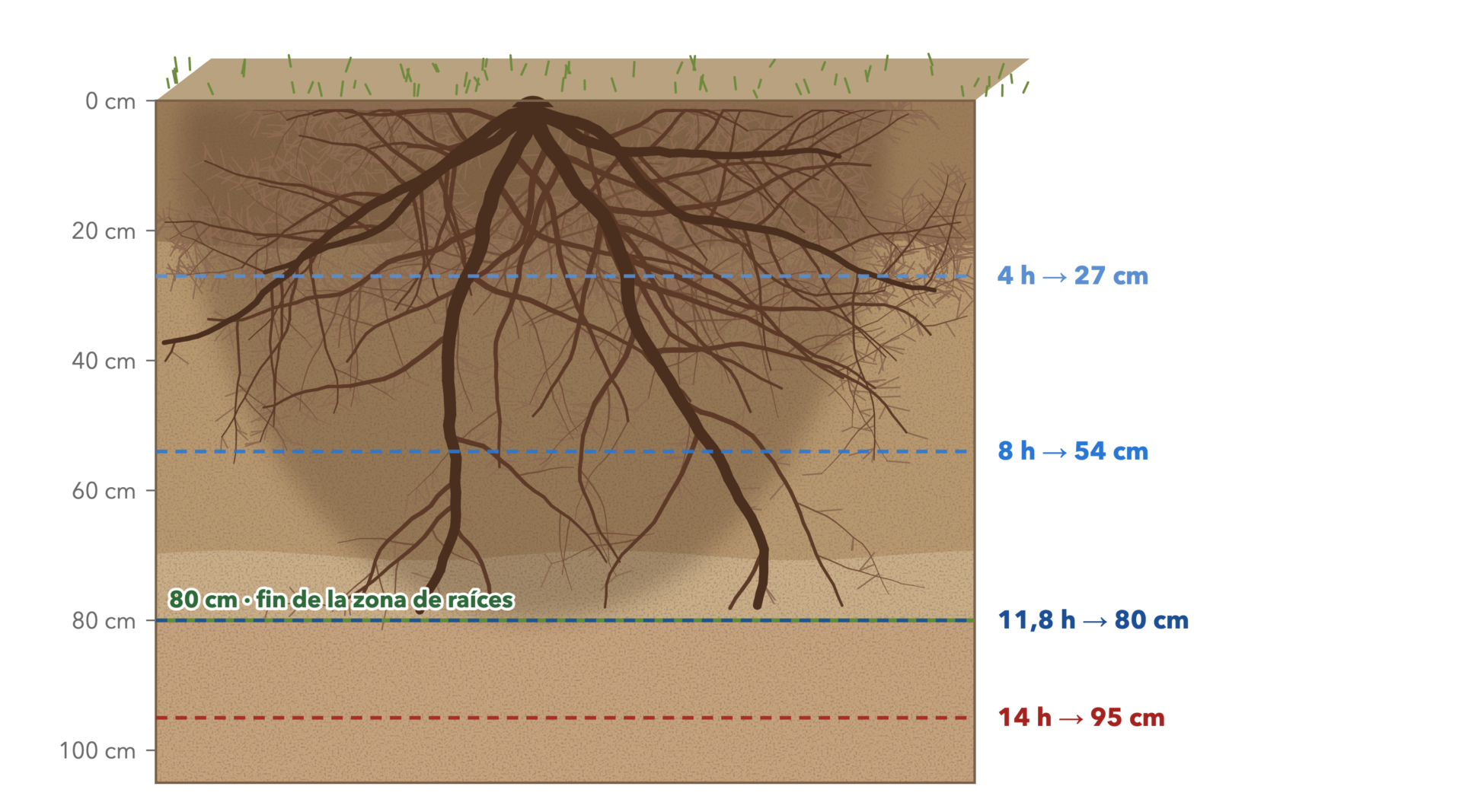
Irrigation duration may need to be increased if the defined depletion threshold—for instance, 40% of available soil moisture—is exceeded. Therefore, monitoring via water balance calculations, probes, and similar tools should always be complemented by the use of soil pits to observe actual conditions within the soil profile.
4. How often should irrigation occur? The water balance approach prevails.
Irrigation frequency is determined by projecting plant water consumption (ETc) against the volume of “readily available” water (within established irrigation criteria) that the soil can store.
In the standard method, reference evapotranspiration (ETo) is calculated using the FAO-56 Penman-Monteith equation. Data must be sourced from a weather station situated under “reference” conditions—representing a hypothetical, actively growing, well-watered grass crop 12 cm tall, with an albedo of 0.23 and a surface resistance of 70 s/m, fully covering the ground (Allen et al., 2006). In practice, this requires the station to be installed over short (8–15 cm), irrigated grass—never over bare soil, gravel, or concrete—in the center of an open, uniform area free from tree shade, and equipped with an anemometer at a height of 2 meters. If the station is surrounded by dry soil, the air becomes warmer than the reference condition, leading to an overestimation of calculated ETo.

To illustrate how frequency works, Figures 3 and 4 use the same soil as in the example (71 mm water-holding capacity) with an average demand of 5.4 mm/day (ETo of 5.4 mm/day and Kc of 1) and irrigation every 4 days using equipment with a 2.0 mm/h application rate and 90% efficiency. Over four days, the orchard consumes 21.6 mm—practically the net depth from the example—bringing the soil right to the irrigation threshold; a 12-hour irrigation (24 mm gross, 21.6 mm effective)—sufficient to reach the effective root depth—restores it to field capacity (Figure 3). Figure 4 uses the same parameters but with 8-hour irrigation cycles (16 mm gross, 14.4 mm effective).
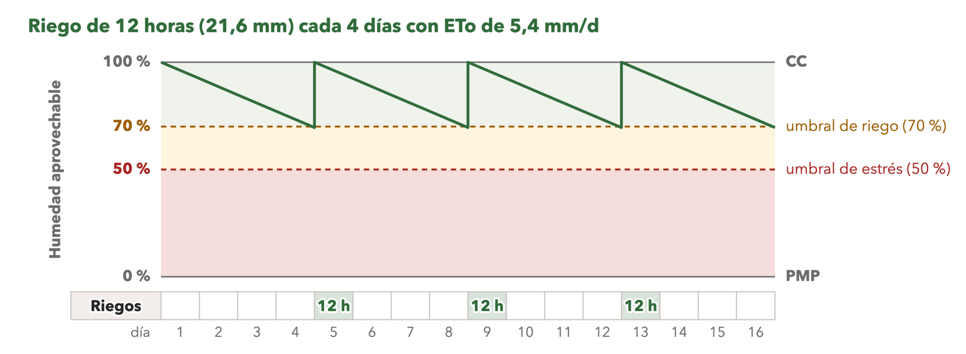
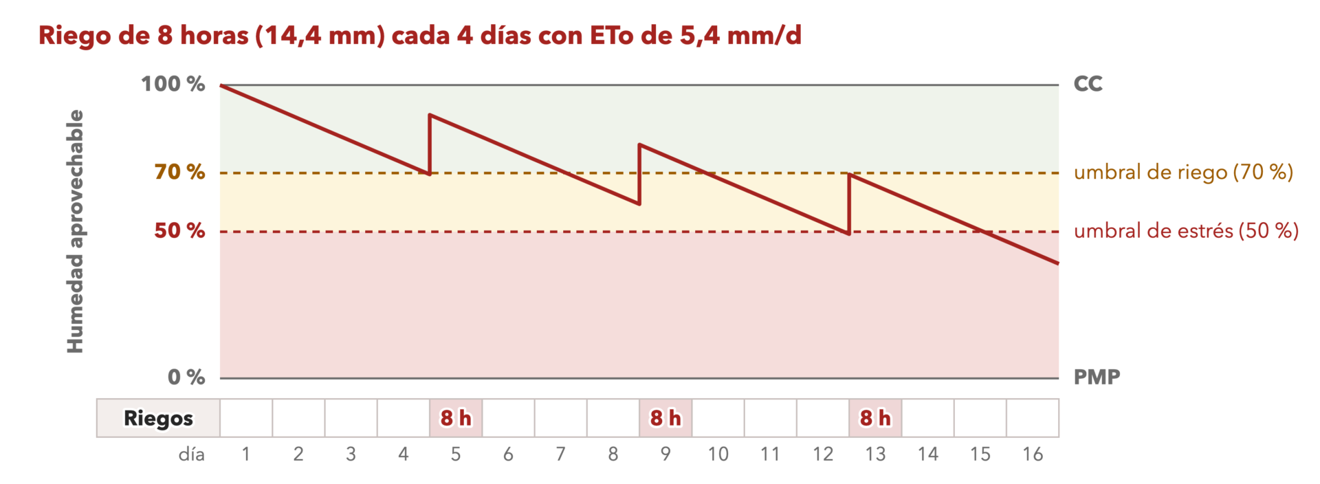
In Figure 3, each irrigation event occurs just as the soil reaches the irrigation threshold (70% of available water) and restores it to field capacity (FC); this is the desired dynamic. In Figure 4, each irrigation event leaves 7.2 mm unreplaced: the soil falls below the irrigation threshold starting from the second cycle, enters a state of stress around day 13, and ends at 39% of available water. To return to FC and resume the dynamic shown in Figure 3, the irrigation event on day 13 would need to replenish 36 mm of effective water (40 mm gross, requiring about 20 hours) instead of the scheduled 8 hours.
In practice, the scenario in Figure 4 is equivalent to skipping an irrigation event: each 8-hour irrigation replenishes only two-thirds of the water consumed (14.4 mm out of 21.6 mm), and the deficit accumulates in the water balance at a rate of 7.2 mm per cycle. By the third irrigation event, the accumulated deficit reaches 21.6 mm—the equivalent of one full irrigation; consequently, the soil dries out progressively, demonstrating that maintaining the frequency does not compensate for insufficient irrigation duration.
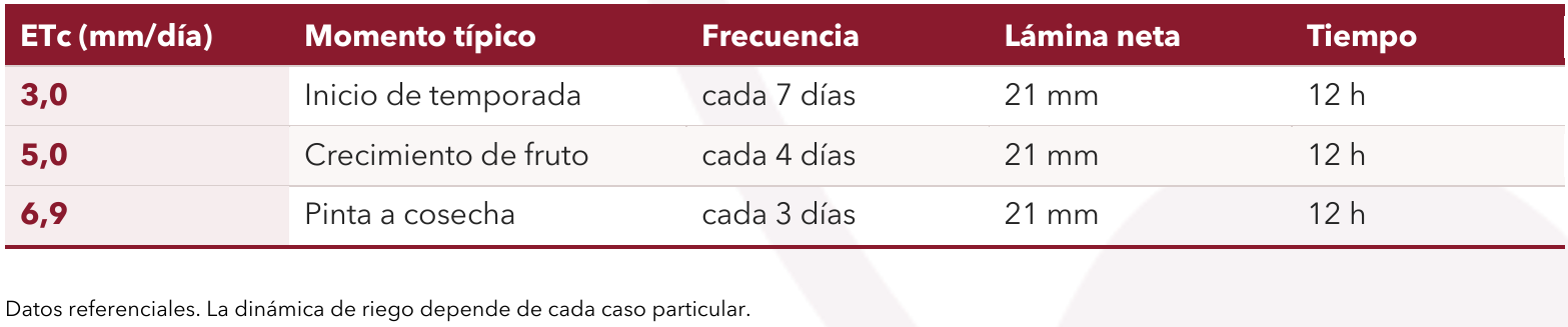
Table 2. Hypothetical frequency and irrigation duration for the example (net depth: 21 mm; gross depth: 24 mm with equipment applying 2.0 mm/h)
5. New technologies for estimating plant water consumption
Technologies currently exist that allow for the measurement or estimation of actual orchard evapotranspiration—such as Eddy Covariance and energy balance models using thermal satellite imagery (e.g., METRIC [Allen et al., 2007] and SEBAL [Bastiaanssen et al., 1998])—which have been validated in Chile for fruit crops like apples (de la Fuente-Saiz et al., 2024). At the plant level, sap flow sensors measure transpiration (rather than soil evaporation) (Granier, 1987), while dendrometers record fluctuations in trunk diameter; maximum daily contraction reflects the plant’s water status rather than water demand, and in cherry trees, this metric has been studied as an indicator for irrigation scheduling (Livellara et al., 2011).
Another widely used methodology involves estimating the crop coefficient via remote sensing, utilizing empirical relationships with vegetation indices such as NDVI (Allen and Pereira, 2009; Kamble et al., 2013). NDVI represents canopy cover and vegetative expression, thereby following the same seasonal dynamics as the crop coefficient (Kc): it rises as leaf area increases, stabilizes at full canopy cover, and declines during the post-harvest period. This explains the relative success of such estimates. However, these complementary technologies must always be cross-checked against soil profile pits to confirm moisture levels and the actual criteria of the irrigation strategy in situ.
Additionally, thermography (via UAV or satellite) estimates foliage temperature, which rises when the plant closes its stomata and transpires less. Therefore, unlike NDVI, it does detect reduced consumption caused by water deficit and allows for the development of coefficients and the adjustment of demand based on a more objective criterion: the orchard’s actual consumption rather than just its potential based on foliage (Gonzalez-Dugo et al., 2013; Carrasco-Benavides et al., 2020).
References
– Allen, R. G. and Pereira, L. S. (2009). Estimating crop coefficients from fraction of ground cover and height. Irrigation Science 28(1): 17-34.
– Allen, R. G., Pereira, L. S., Raes, D. and Smith, M. (2006). Crop evapotranspiration: guidelines for computing crop water requirements. FAO Irrigation and Drainage Paper 56. FAO, Rome.
– Allen, R. G., Tasumi, M. and Trezza, R. (2007). Satellite-based energy balance for mapping evapotranspiration with internalized calibration (METRIC)—Model. Journal of Irrigation and Drainage Engineering 133(4): 380-394.
– Bastiaanssen, W. G. M., Menenti, M., Feddes, R. A. and Holtslag, A. A. M. (1998). A remote sensing surface energy balance algorithm for land (SEBAL). 1. Formulation. Journal of Hydrology 212-213: 198-212.
– Carrasco-Benavides, M. et al. (2020). Performance assessment of thermal infrared cameras of different resolutions to estimate tree water status from two cherry cultivars: an alternative to midday stem water potential and stomatal conductance. Sensors 20(12): 3596.
– De la Fuente-Saiz, D., Ortega-Farías, S., Carrasco-Benavides, M. et al. (2024). Assessment of satellite-based water requirements for a drip-irrigated apple orchard in Mediterranean agroclimatic conditions. Heliyon 10: e29688.
– Gonzalez-Dugo, V., Zarco-Tejada, P., Nicolás, E. et al. (2013). Using high resolution UAV thermal imagery to assess the variability in the water status of five fruit tree species within a commercial orchard. Precision Agriculture 14(6): 660-678.
– Granier, A. (1987). Evaluation of transpiration in a Douglas-fir stand by means of sap flow measurements. Tree Physiology 3(4): 309-320.
– Kamble, B., Kilic, A. and Hubbard, K. (2013). Estimating crop coefficients using remote sensing-based vegetation index. Remote Sensing 5(4): 1588-1602.
– Livellara, N., Saavedra, F. and Salgado, E. (2011). Plant based indicators for irrigation scheduling in young cherry trees. Agricultural Water Management 98(4): 684-690.
– Saxton, K. E. and Rawls, W. J. (2006). Soil water characteristic estimates by texture and organic matter for hydrologic solutions. Soil Science Society of America Journal 70(5): 1569-1578.